
Appearance
Visualisation of the Alpha algorithm
This algorithm was the first algorithm proposed for the construction of a Petri net from an event log. It has been built on a lot since to be generalised for more event log attributes and a variety of other complexities.
Requirements
The event log
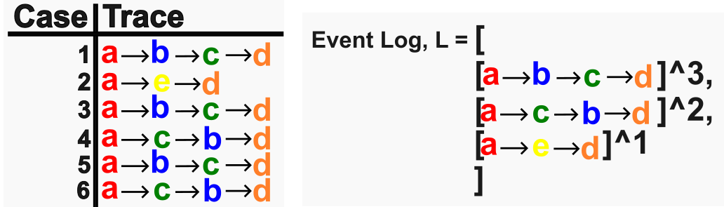
Process discovery begins with an event log which in its simplest form is a table with columns of activity, timestamp and case. If we sort by timestamp and then filter by case we can easily extract traces (individual end to end process instances) by just looking at the activity column.
The footprint matrix
We can generate a table that shows the pairwise relationship between activities.
- X->Y means Y sometimes directly follows X but X never follows Y
- X<-Y means X sometimes directly follows Y but Y never follows X
- X#Y and Y#X means there is no directly follows relationship
- X||Y or Y||X means sometimes X directly follows Y and sometimes Y directly follows X
This is called the footprint matrix:
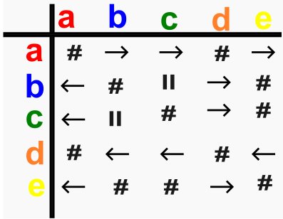
While the footprint matrix is not strictly required to be defined mathematically for the algorithm, it is practically helpful for the implementation.
The algorithm
Extracting the activity relations
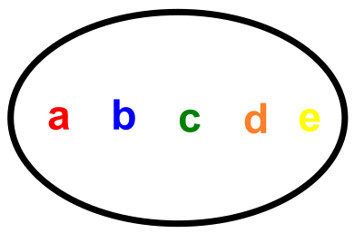
1. Unique activities
We need to define a set that contains one instance of each of the activities that occurred one or more times.
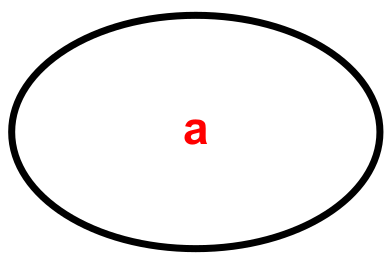
2. Start activities
We need to define a set that contains one instance of each of the activities that occurred at the start of a trace one or more times.
3. End activities
We need to define a set that contains one instance of each of the activities that occurred at the end of a trace one or more times.
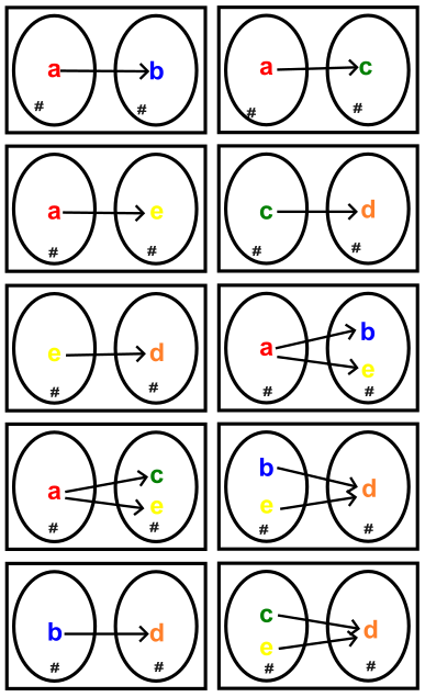
4. Related pairs of independent sets
Now, we need to construct pairs of sets where:
- All the elements in each set are a subset of the set of unique activities (remember step 1 of the algorithm).
- The elements within each set are independent of each other.
- All elements in one set are dependent on one or more elements in the other set in the pair.
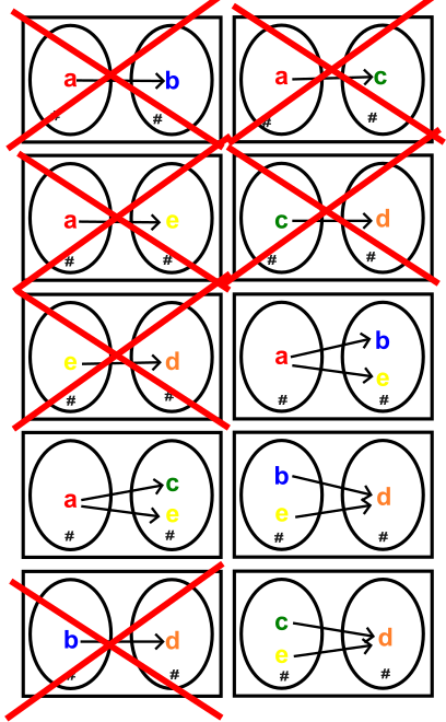
5. Drop non maximal pairs of sets
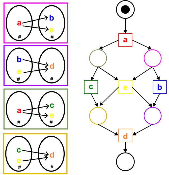
Looking at the figure of all the related pairs of independent sets it is clear that many of them are combinations of the others. A non-maximal pair of sets is one that can be combined with another set to form a pair we already have. We can throw these away since they don't contain additional information.
Drawing the Petri net
6. Drawing places, transitions and relations
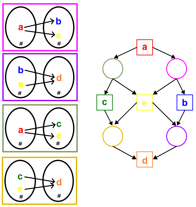
Each one of the maximal pairs of sets we kept in step 5 of the algorithm now become a place/state in our Petri net. We create a transition/activity on the diagram for each activity in the set of unique activities.
Then, iterating over the pairs of sets that each correspond to a place/state in the Petri net:
- Each activity in the first set of the pair is a pre-cursor to the place that the pair corresponds to (arrow that goes out from the transition to the state)
- Each activity in the second set of the pair is a dependent on the place that the pair corresponds to (arrow that comes into the transition from the state)
7. Adding the start and end
Using the sets of start and end activities, we can finally link these to the start and end virtual places.
References
- The specific example and simple understanding of the algorithm can be found in Study Conquest - Alpha Algorithm (Process Discovery Method)
- Deeper mathematical understanding can be found in Wil M. P. van der Aalst - Process Mining Handbook